Preparation for IC25 and IC50 Estimation
As with all statistical analysis of toxicity data, it is critical to visualize the experimental data distribution through graphing.
A minimum of three replicates is necessary in a toxicity test to enable the calculation of IC25 and IC50.
ToxGenie automatically identifies user-input data and selects the optimal model from among exponential, Gompertz, hormesis, linear, and logistic models for analysis. Therefore, you only need to input your experimental data.
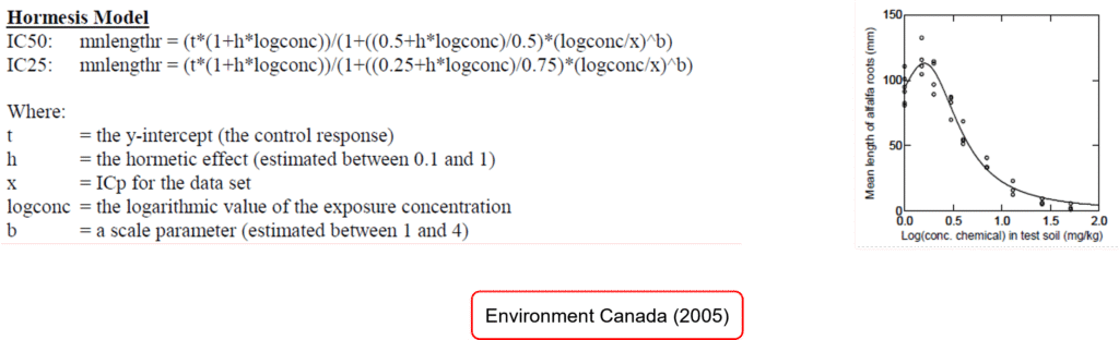
What is the Hormesis Model?
The Hormesis model is a mathematical model widely used in toxicology, biology, and pharmacology to describe the biological response (e.g., inhibition rate, growth rate) to varying concentrations (doses) of a substance. Its defining characteristic is its ability to capture a nonlinear pattern where low concentrations stimulate a biological response, while high concentrations inhibit it. In simple terms, the model reflects the concept that “a small amount is beneficial, but a large amount is harmful.”
Characteristics of the Hormesis Model
U-Shaped or J-Shaped Curve
The Hormesis model typically produces a U-shaped or J-shaped curve. At low concentrations, the biological response (e.g., cell growth, survival rate) is enhanced (stimulated), but as concentrations increase, the response decreases (inhibited) or becomes toxic. For example, this model effectively describes scenarios where small amounts of a substance, such as a vitamin or chemical, may be beneficial, while excessive amounts are harmful.
Nonlinear Response
Unlike linear models, which assume a straight-line relationship, or simple sigmoidal models (e.g., Gompertz or logistic), the Hormesis model accounts for a complex pattern where a positive effect at low concentrations transitions to a negative effect at higher concentrations.
Mathematical Representation
The Hormesis model can be expressed in various mathematical forms, but a common representation is (Environment Canada, 2005):
Comparison with Other Models
- The Gompertz model typically produces an S-shaped curve, describing a response that increases gradually and then plateaus, without accounting for stimulation at low concentrations.
- The Weibull model offers flexibility in curve shape above and below the inflection point but does not explicitly model the stimulatory effect at low concentrations as the Hormesis model does.
Advantages of the Hormesis Model
- Realistic Representation: It accurately models the “low-dose stimulation, high-dose inhibition” phenomenon commonly observed in biological systems.
- Flexibility: The model accommodates U-shaped or J-shaped response patterns, making it versatile for various nonlinear datasets.
- Practical Utility: It helps distinguish between safe (beneficial) and harmful concentration ranges for toxic substances or drugs.
Limitations of the Hormesis Model
- Data Requirements: Accurate modeling requires sufficient data points at both low and high concentrations, particularly to capture the stimulatory effect at low doses.
- Complexity: The model is mathematically more complex than linear models, often requiring computational tools (e.g., ToxGenie) to estimate parameters.
- Applicability: The Hormesis model may not be suitable if the data do not exhibit a U-shaped or J-shaped pattern.
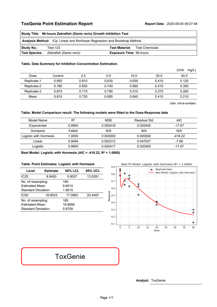
Analysis Results of ToxGenie’s IC25 and IC50 Estimation
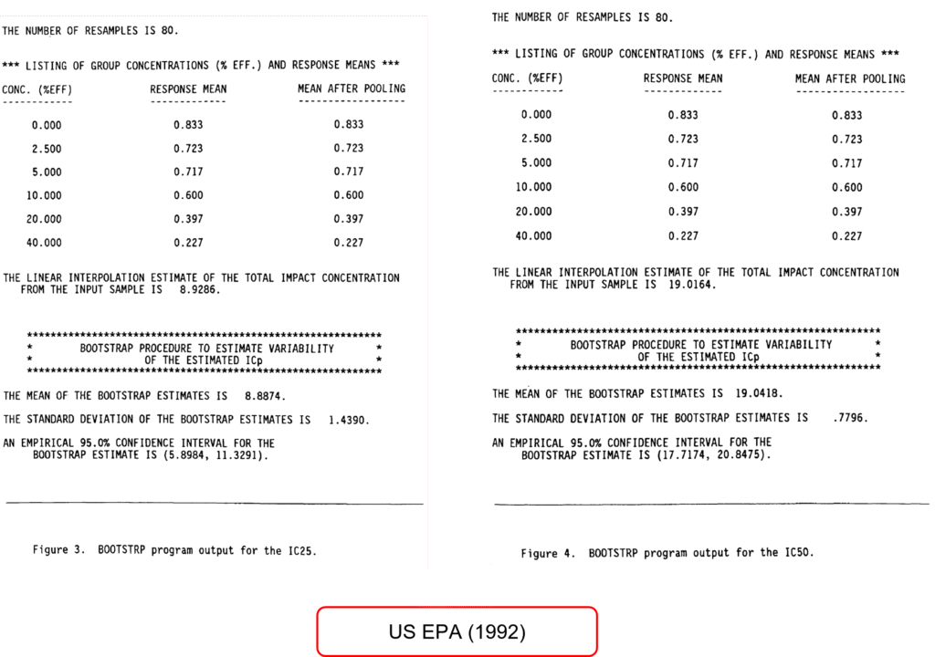
To compare ToxGenie’s analysis results, IC25 and IC50 estimation methods were applied using the same data as in the US EPA Report (EPA/600/4-91/021, February 1992). The results are shown above. However, due to difficulties in obtaining data optimized for each model, representative analysis results are provided, and users are encouraged to analyze various datasets.
The US EPA used the Linear Interpolation method to calculate IC25 and IC50, with 80 resamples. However, Environment Canada (2005) recommends a minimum of 240 resamples. ToxGenie employs 240 resamples, excluding outlier data, to calculate 95% confidence limits. Consequently, there are slight differences from the US EPA results, but all fall within the 95% confidence interval. The reasons for these differences are explained below.
The US EPA’s Linear Interpolation method estimates IC25 and IC50 values through simple linear interpolation, relying on linear connections between data points. This approach is fast and intuitive but may fail to capture nonlinear biological responses (e.g., sigmoidal curves). In contrast, exponential, Gompertz, hormesis, linear, and logistic models use nonlinear regression analysis to model more complex dose-response relationships.
Resampling 80 times estimates 95% confidence limits through bootstrapping but may not fully capture the variability of the distribution due to the small sample size, potentially resulting in less stable confidence limits. Resampling 200 or more times reflects the distribution’s characteristics more accurately, narrowing the confidence interval and increasing stability.
Start Your Toxicity Data Statistical Analysis with ToxGenie
Understanding quantal and quantitative data is the first step toward robust toxicology research. ToxGenie offers an intuitive platform for both data types, suitable for beginners and experts alike. Curious? Start with a 30-day free trial and revolutionize your toxicity data statistical analysis today!